From distance matrix to binary tree
In one of our current exercises we have to prove different properties belonging to distance matrices as base of binary trees. Additionally I tried to develop an algorithm for creating such a tree, given a distance matrix.
A distance matrix \(D \in \mathbb{R}^{N,N}\) represents the dissimilarity of \(N\) samples (for example genes), so that the number in the i-th row j-th column is the distance between element i and j. To generate a tree of it, it is necessary to determine some attributes of the distance \(d(x,y):\mathbb{R}^n \times \mathbb{R}^n \rightarrow \mathbb{R}\) between two elements so that it is a metric:
- \(d(x, y) \ge 0\) (distances are positive)
- \(d(x, y) = 0 \Leftrightarrow x = y\) (elements with distance 0 are identical, dissimilar elements have distances greater than 0)
- \(d(x, y) = d(y, x)\) (symmetry)
- \(d(x, z) \le d(x, y) + d(y, z)\) (triangle inequality)
Examples for valid metrics are the euclidean distance \(\sqrt{\sum_{i=1}^n (x_i-y_i)^2}\), or the manhattan distance \(\sum_{i=1}^n \|x_i-y_i\|\).
The following procedure is called hierarchical clustering, we try to combine single objects to cluster. At the beginning we start with \(N\) cluster, each of them containing only one element, the intersection of this set is empty and the union contains all elements that should be clustered.
The algorithm now searches for the smallest distance in \(D\) that is not 0 and merges the associated clusters to a new one containing all elements of both. After that step the distance matrix should be adjusted, because two elements are removed and a new one is added. The distances of the new cluster to all others can be computed with the following formula:
\[d(R, [X+Y]) = \alpha \cdot d(R,X) + \beta \cdot d(R,Y) + \gamma \cdot d(X,Y) + \delta \cdot |d(R,X)-d(R,Y)|\]\(X, Y\) are two clusters that should be merged, \(R\) represents another cluster. The constants \(\alpha, \beta, \gamma, \delta\) depend on the cluster method to use, shown in table 1.
| Method | $$\alpha$$ | $$\beta$$ | $$\gamma$$ | $$\delta$$ |
|---|---|---|---|---|
| Single linkage | 0.5 | 0.5 | 0 | -0.5 |
| Complete linkage | 0.5 | 0.5 | 0 | 0.5 |
| Average linkage | 0.5 | 0.5 | 0 | 0 |
| Average linkage (weighted) | $$\frac{|X|}{|X| + |Y|}$$ | $$\frac{|Y|}{|X| + |Y|}$$ | 0 | 0 |
| Centroid | $$\frac{|X|}{|X| + |Y|}$$ | $$\frac{|Y|}{|X| + |Y|}$$ | $$-\frac{|X|\cdot|Y|}{(|X| + |Y|)^2}$$ | 0 |
| Median | 0.5 | 0.5 | -0.25 | 0 |
Here \(\|X\|\) denotes the number of elements in cluster \(X\).
The algorithm continues with searching for the smallest distance in the new distance matrix and will merge the next two similar elements until just one element is remaining.
Merging of two clusters in tree-view means the construction of a parent node with both clusters as children. The first clusters containing just one element are leafs, the last node is the root of the tree.
Small example
Let’s create a small example from the distance matrix containing 5 clusters, see table 2.
| A | B | C | D | E | |
|---|---|---|---|---|---|
| A | 0 | 5 | 2 | 1 | 6 |
| B | 5 | 0 | 3 | 4 | 1.5 |
| C | 2 | 3 | 0 | 1.5 | 4 |
| D | 1 | 4 | 1.5 | 0 | 5 |
| E | 6 | 1.5 | 4 | 5 | 0 |
A and D are obviously the most similar elements in this matrix, so we merge them. To make the calculation easier we take the average linkage method to compute the new distances to other clusters:
\(d(B,[A+D]) = \frac{d(B, A) + d(B, D)}{2} = \frac{5 + 4}{2} = 4.5\)
\(d(C,[A+D]) = \frac{d(C, A) + d(C, D)}{2} = \frac{2 + 1.5}{2} = 1.75\)
\(d(E,[A+D]) = \frac{d(E, A) + d(E, D)}{2} = \frac{6 + 5}{2} = 5.5\)
With these values we are able to construct the new distance matrix of 4 remaining clusters, shown in table 3.
| A,D | B | C | E | |
|---|---|---|---|---|
| A,D | 0 | 4.5 | 1.75 | 5.5 |
| B | 4.5 | 0 | 3 | 1.5 |
| C | 1.75 | 3 | 0 | 4 |
| E | 5.5 | 1.5 | 4 | 0 |
This matrix gives us the next candidates for clustring, B and E with a distance of 1.5.
\(d([A+D], [B+E]) = \frac{d([A+D], B) + d([A+D], E)}{2} = \frac{4.5 + 5.5}{2} = 5\)
\(d(C,[B+E]) = \frac{d(C, B) + d(C, E)}{2} = \frac{3 + 4}{2} = 3.5\)
With the appropriate distance matrix of table 4.
| A,D | B,E | C | |
|---|---|---|---|
| A,D | 0 | 5 | 1.75 |
| B,E | 5 | 0 | 3.5 |
| C | 1.75 | 3.5 | 0 |
Easy to see, now we cluster [A+D] with C:
\[d([B+E], [A+C+D]) = \frac{d([B+E],C) + d([B+E],[A+D])}{2} = \frac{3.5+5}{2} = 4.25\]and obtain a last distance matrix with table 5.
| A,C,D | B,E | |
|---|---|---|
| A,C,D | 0 | 4.25 |
| B,E | 4.25 | 0 |
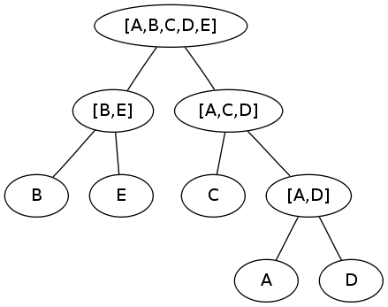
Needless to say, further calculations are trivial. There are only to clusters left and the combination of them gives us the final cluster containing all elements and the root of the desired tree.
The final tree is shown in figure 1. You see, it is not that difficult as expected and ends in a beautiful image!
Remarks
If \(D\) is defined as above there is no guarantee that edge weights reflect correct distances! When you calculate the weights in my little example you’ll see what I mean. If this property is desired the distance function \(d(x,y)\) has to comply with the condition of ultrametric inequality: \(d(x, z) \le \max {d(x, y),d(y, z)}\).
The method described above is formally known as agglomerative clustering, merging smaller clusters to a bigger one. There is another procedure that splits bigger clusters into smaller ones, starting with a cluster that contains all samples. This method is called divisive clustering.

Leave a comment
There are multiple options to leave a comment: